Interest Rate Models
Interest Rate Models (IRMs) determine borrow and supply rates based on market conditions. They are the pricing mechanism for capital in lending markets.How IRMs Work
Every lending market needs a mechanism to balance supply and demand. IRMs solve this by adjusting rates based on utilization:- When utilization is high (more borrowing demand), rates increase to attract suppliers and discourage borrowing
- When utilization is low (excess supply), rates decrease to encourage borrowing
Types of IRMs
Rosetta tracks markets across protocols that use different IRM architectures. 1- Fixed Curve Models Rates follow a predefined curve with parameters set by governance. Typically a piecewise-linear function with a “kink” at optimal utilization, where rates begin increasing more steeply. 2- Adaptive Models (Morpho) Rates follow a curve that adjusts itself over time based on market behavior. If utilization consistently runs above target, the curve shifts upward. If utilization runs below target, it shifts downward. Used by Morpho markets on both HyperEVM and Base. The Adaptation The target rate (r₉₀%) itself shifts over time:- If utilization stays above 90%, r₉₀% gradually increases, pushing rates higher to attract more supply and discourage borrowing
- If utilization stays below 90%, r₉₀% gradually decreases, lowering rates to encourage borrowing
- Below optimal utilization: rates increase gradually along a base slope
- Above optimal utilization: rates increase steeply along a second slope to incentivize repayment
Borrow APY = e^(borrowRate × secondsPerYear) − 1
Supply APY is derived from Borrow APY, scaled by utilization:
Supply APY = Borrow APY × Utilization × (1 − Protocol Fee)
Suppliers earn a share of borrower interest proportional to how much of the pool is actively borrowed. This formula applies to both Morpho and Aave markets.
The APY Problem
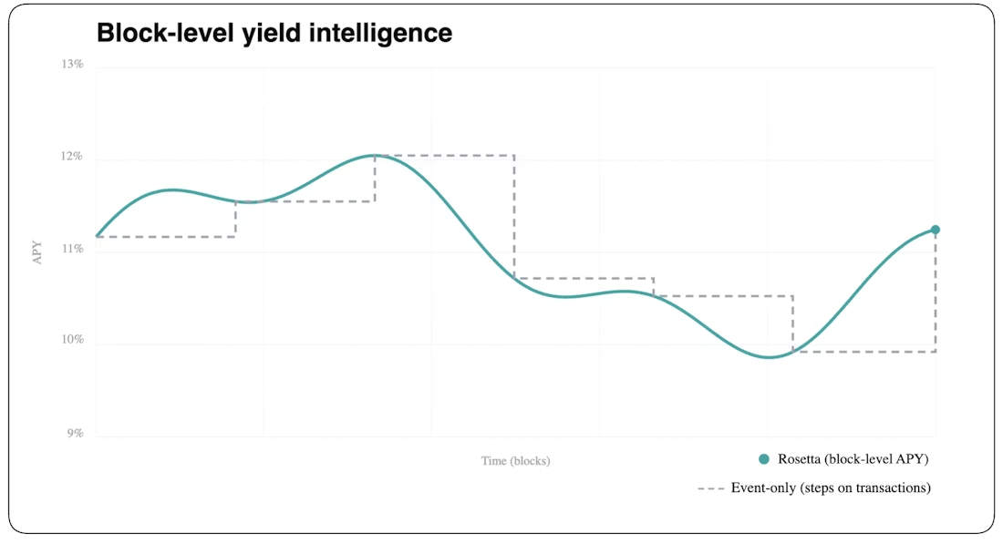
APY displayed on most interfaces does not reflect what users actually earn.Event-Based Updates
Most dashboards update yield figures only when transactions occur: deposits, withdrawals, borrows, repayments. Between transactions, the displayed APY remains static. But interest accrues continuously. Every block, borrowers owe more and lenders are entitled to more. A dashboard showing 5.00% might be displaying a value from hours or days ago, while the actual rate has shifted with utilization. Displayed APY = Rate at last transaction Actual APY = Rate at current block Quick example:13:02:00— Event‑based UI shows 12.8%.13:02:15— Utilization softens (no tx); model implies 11.9%.13:02:16— Rosetta already shows 11.9%.13:03:40— First tx lands; event‑based UI finally updates to 11.9%.
Market Impact
The APY you see before depositing is not the APY you get after. Your deposit changes the market:- Depositing into a market increases supply, lowering utilization, lowering rates
- Depositing into a vault triggers allocation, potentially spreading impact across markets